Numerics on Exponential Sums

14th April 2015

Here we outline some of the numerical aspects of arXiv:1408.5743 in more detail. We lead in to the results through a discussion of more classical topics. Apart from just providing the programs relevant to the paper, this article aims to give some insight into how we expected to arrive at the final result. In the end, a list of all the relevant data is provided. The list of eigenvalues used in the computations was adapted from the data of H. Then (Maass cusp forms for large eigenvalues, Math. Comp. 74 (2005) 363–381) which was provided under the Creative Commons Attribution-Noncommercial-Share Alike 3.0 Unported License. The list is available here.

Let $\zeta$ be the Riemann zeta function and denote its non-trivial zeros by $\rho=\beta+i\gamma$ . In 1912, Landau proved the following striking result for an exponential sum related to the zeros:

Landau’s Formula Fix $x>1$ , then, as $T\rightarrow\infty$ , we have:

$\displaystyle\sum_{\gamma\leq T}x^{\rho}=-\frac{T}{2\pi}\Lambda(x)+O(\log T).$

Here $\Lambda$ is the von Mangoldt function which is defined as $\Lambda(x)= \log p$ if $x=p^{m}$ , for some prime p, and is 0 otherwise. Therefore, the exponential sum grows by an order of T precisely when x is a power of a prime. This means that we can use the sum as a (inefficient) way of detecting primes. Perhaps it is also unexpected that the proof of this formula follows from a fairly elementary contour integration and some estimates on the growth of the Riemann zeta function. However, underneath the surface there is a deeper connection arising from the Weil explicit formula for the zeta function, which in turn is a consequence of the Euler and Hadamard products of $\zeta$ as well as the functional equation (which is essentially Poisson summation for appropriately chosen test function). I will write a separate post on this later.

With the data of Odlyzko for the heights of the zeros of $\zeta$ , it is easy to construct a Python script to verify this theorem (note in order to run this code you need mpmath and matplotlib and their dependencies). We obtain the following (normalised) plot which shows the real part of the sum in blue and the imaginary part in green: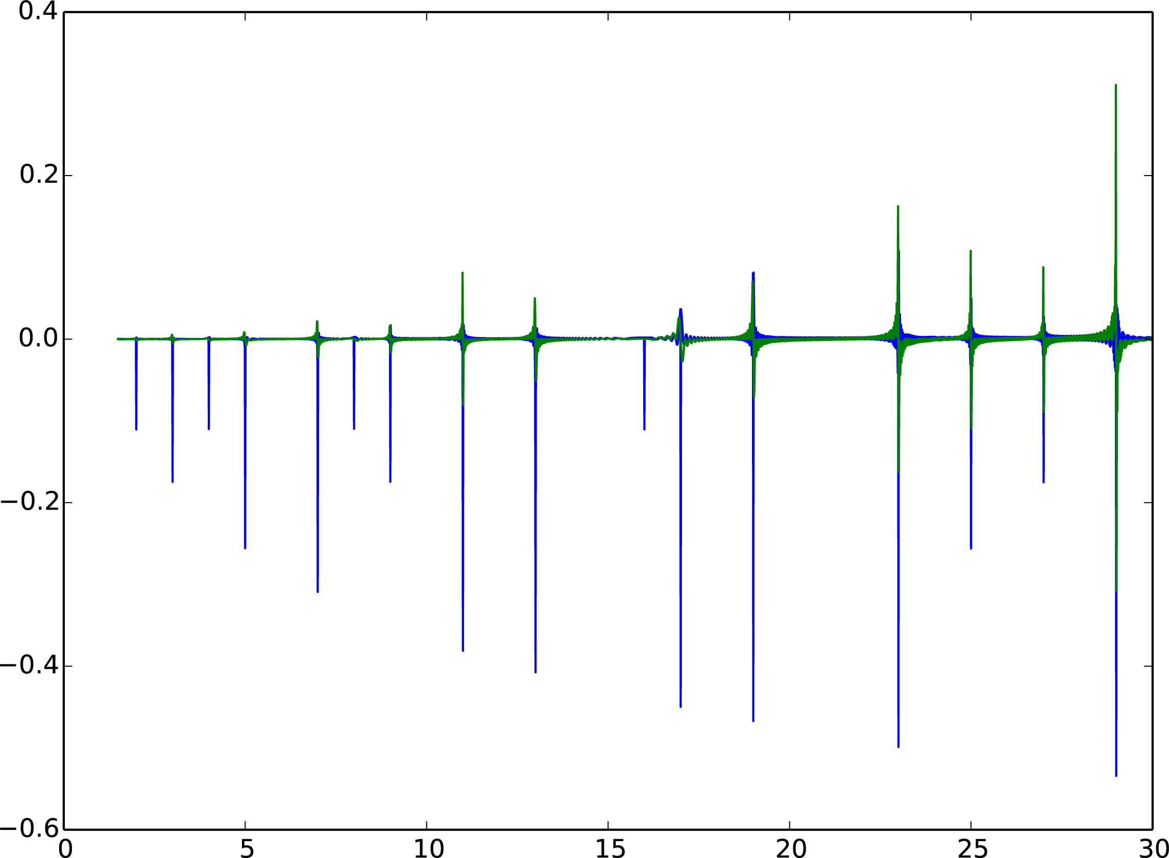
Of course, if we extended the sum to the negative zeros, then the imaginary part would be trivially zero. The above picture seems to agree with the Landau Formula as there are peaks at all prime powers. Another thing to note, which one might not have expected after a quick inspection of Landau’s formula, is that the peaks at actual primes are significantly larger than at higher powers. This is simply because $\Lambda$ is constant on powers of a fixed prime, so that any peak that is higher than the preceding ones necessarily corresponds to a new prime.

Now, recall that the original intent of this post was to examine the behaviour of the exponential sum $S(T,X)$ defined by

$S(T,X)=\displaystyle\sum_{|t_{j}|\leq T}X^{i t_{j}},$
where $X>1$ and the spectral parameters $t_{j}$ come from the eigenvalues $\lambda_{j}=\frac{1}{4}+t_{j}^{2}$ of the Laplacian $\Delta$ on $M=\mathrm{PSL}_{2}(\mathbb{Z})\backslash\mathbb{H}$ . The conjecture is that this sum exhibits square root cancellation, giving $S(T,X)\ll_{\epsilon}T^{1+\epsilon}X^{\epsilon}$ .

Our $S(T,X)$ is not completely analogous to the exponential sum in Landau’s formula as we are summing over both the positive and negative parameters so that the imaginary part (the sine kernel) vanishes. It turns out to be a bit more difficult to prove any results for the general case. We can, however, investigate this with numerical computations as before. There is limited public data available for the eigenvalues. Nevertheless, we adapt our Python script to investigate the behaviour of $S(T,X)$ (and the corresponding sum for sine) in terms of T or X.

The more interesting case occurs when we fix a large T and vary X. In the same way that we saw the peaks at prime powers for the $\zeta$ , we expect to be able to decipher some main terms in this case as well. With this Python script we obtain, for example, the following plot (where, as before, blue and green represent the real and imaginary parts, respectively):

Initially, we expect to see growth at the lengths of the closed geodesics of M (in short, because $S(T,X)$ is essentially the heat kernel on M which follows the geodesic flow of M). For example, in the above picture the peaks at $X=6.854\ldots,\,X=13.928\ldots$ correspond to closed geodesics. We can notice a few other interesting phenomena here.

First of all, there is another peak at $X=9$ that is not explained by the geodesics. With further plots we identify similar peaks at 16, 25, 49, 64 and so on. This suggests (a somewhat surprising) behaviour at even prime powers. In the paper we explain how this arises from the continuous spectrum of $\Delta$ . On top of that, the oscillations in $S(T,X)$ seem to be much stronger than in the classical case, which leads one to suspect that the main term should have an oscillatory component. We will look at this in more detail in the T-plots. First let us look at another plot for a smaller range of X:

Now we see the oscillations more clearly. Firstly, the oscillations in the real and imaginary parts agree and are just slightly out of sync. This is not unexpected. However, at peak points, something uncharacteristic happens: while the real part (blue) has a large peak only on positive values, the imaginary part (green) has slightly smaller peaks for both negative and positive values around the actual X coordinate for the peak. Moreover, precisely at the peak point the sine kernel seems to vanish. These are recurring phenomena for all the peak points we could find.

We can also fix an X and plot the values of the exponential sum for increasing T. This allows us to investigate the stability of the sum in terms of T and also to say something more about the oscillations that are occurring. First, let us look at plots at a peak point and away from one. We will focus on the peaks arising from the prime geodesics, because, as we’ll see later, the peaks at even prime powers fade out for large X.

Here we are close to the peak point $X=46.9787\ldots$ . As we saw before, the imaginary part (green) concentrates around 0, while the peak comes from the real part. Both sums, though, seem to achieve their respective asymptotics fairly quickly, and already after $T=200$ there is hardly any movement. Let’s look at a different example.

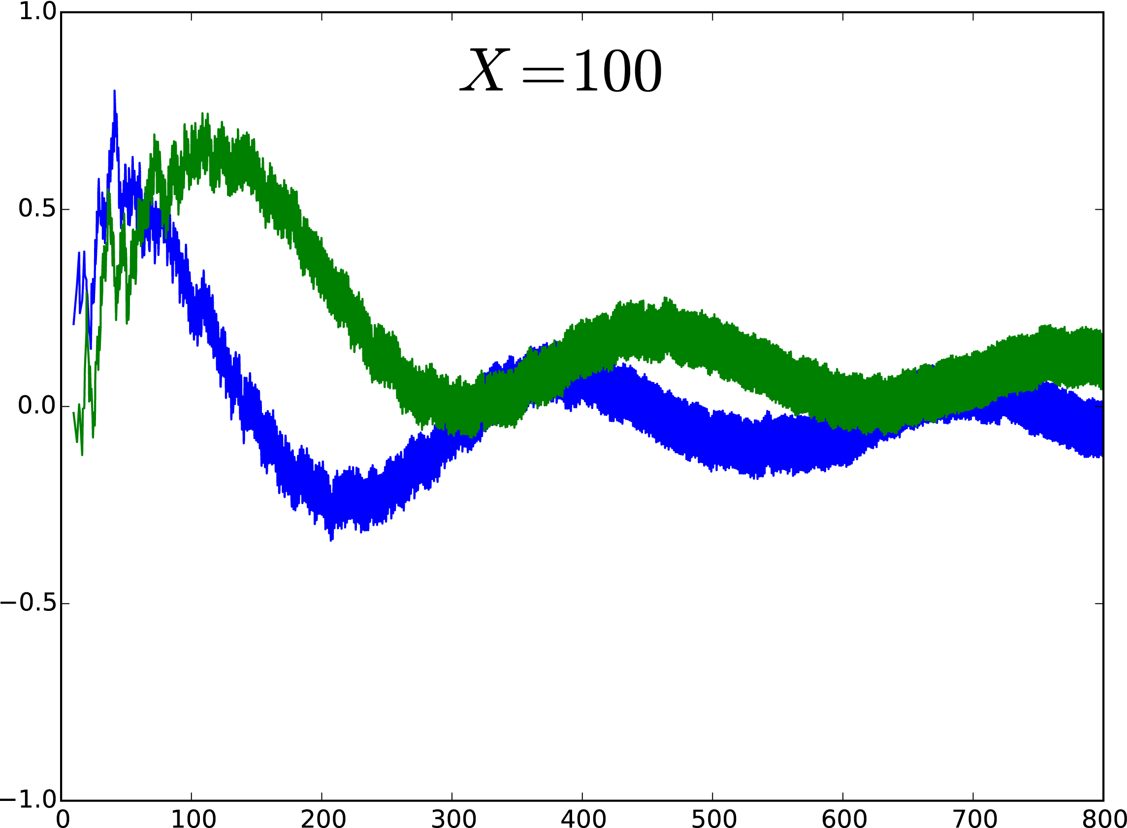
Now we are not at a peak point, so we see steady oscillation in terms of T. Notice that there seems to be a mix of two very different oscillations. One local one, with a very short period, which is responsible for the roughness of the graph. The other oscillatory component is easier to spot since the period is very large in T. One interesting point to note (and this is easier to see in an animation, VLC is recommended for viewing) is that this large period seems to shrink and grow depending on whether we are close to a peak point or far away, respectively. One might argue this is because at peak points this large oscillation is killed off as we saw above.

Finally, we can zoom in an investigate the small oscillations (by small I mean the amplitude even if the actual wave is located at a high value, like what happens at peak points). Here we have concentrated around $500<T<510$ for $X=23.14\displaystyle\approx e^{\pi}$ .

We see that there is one period between 504 and 506. Squaring the X value we arrive at $X=535.491$ .

Now we have two period between 504 and 506. This suggest that the oscillatory term of T has logarithmic dependance on X.

We now note that many of the above phenomena (for example why the even prime power peaks fade away) can be seen from the theorem that was proven in the paper:

Theorem 1 (L 2014) Fix $X>1$ , then, as $T\rightarrow\infty$ , we have

$S(T,X)=\displaystyle\frac{|F|}{\pi}\frac{\sin(T\log X)}{\log X}T+\frac{T}{\pi}(X^{1/2}-X^{-1/2})^{-1}\Lambda_{\Gamma}(X)+\frac{2T}{\pi}X^{-1/2}\Lambda(X^{1/2})+O(T/\log T).$

Here $|F|$ is the volume of the fundamental domain of $\Gamma$ , $\Lambda$ is the usual von Mangoldt function and $\Lambda_{\Gamma}$ is its generalisation to lengths of closed geodesics. The proof is an application of the Selberg Trace Formula (which is an analogue of the Poisson Summation formula mentioned earlier, which is also a simple trace formula in itself!) for a carefully chosen test function.

Some more numerics were done that are not yet discussed in this post. For example, it is possible predict the square root cancellation in T (in the above discussion we just assumed we knew the normalisation should be T). Also, while the above computations were carried to a relatively high precision, it turns out that truncating the eigenvalues does not have a huge effect on the asymptotics (at least in the range we are working in). We used eigenvalues with precisions 30, 10 and 2 for this investigation. It is also possible to subtract the oscillatory main term found in Theorem 1. This provides a way of investigating the other oscillations more precisely. This is incorporated in the Python programs.

There are many questions left unanswered though:

The oscillations at peak points for the sine and cosine kernels seem to be of different nature, why?
Moreover, the overall nature of the oscillations is still a mystery: why do the large oscillations become more rapid only to die off at peak points?
We can find frequent locations, with no obvious pattern, where the modulus of the sum becomes really small inside an interval of significant length. What is going on there?
Why is the summation so stable in T? We only seem to need about $T\approx 80$ , to get fairly accurate results (same for the precision of the eigenvalues).

As a conclusion, here is a convenient list of all the data provided in this post: